Video Tutorial Library

In the first of this new series of video tutorials the features and functions of the Boddies Extreme (BEX) surface analysis software are demonstrated and explained.
The series begins here with an introduction on how to load data and orientate yourself with the main parts of the user interface.
We hope you find this series of tutorials useful, and please feel free to contact us with any feedback or requests you may have.

In Tutorial 2 we explore the main features of the “Image Space” and “Colour Space” areas of the BEX software interface.
We explain how to tilt, pan and zoom the Image Space, while changing between Perspective, Plan (top down) and Orthographic views.
The Colour Space is then used to change the colour scale that represents the surface height, to control how we visualise the surface data.
Finally we manipulate the height (or Z axis) scale to show the surface features.

Tutorial 3 shows how we apply different colour scales surface height data. The Contour tool is introduced and used to better visually represent the Plan view, much like a conventional map.
The colour scale controls are used to fix the upper and lower limits of the height. The are then used as a tool to isolate a range of surface heights and isolate (or cut off) specific parts of the surface data.

Tutorial 4 – here we use tools to automate fitting a reference geometry on multiple individual data sets so they can be viewed comparatively.
We move from a single data set where many of the pyramid features have been measured together in low spatial resolution, to multiple data sets where individual pyramid peaks have been measured in isolation but to much higher spatial resolution.
*Spatial resolution is the distance between surface height measurements e.g. every 100 um gives a low spatial resolution of 10 points per mm, while measurements every 1 um gives a higher spatial resolution of 1000 points per mm.

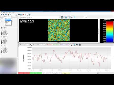
In this video we demonstrate the loading of other data formats including data from AFM (Atomic Force Microscope) measurement systems and stereolithography files (.STL) from X-CT (X-ray Computer Tomography)

This tutorial introduces quantitatively describing complex surfaces. Using 2D cross sections of the 3D surface we show how to determine the distance between features such that height or width of features can be calculated.

In the 7th tutorial we introduce and explain the meaning the commonly used R series of 2D roughness parameters.
Ra (arithmetic absolute mean roughness)
Rq (root mean square roughness)
Rp (highest peak height)
Rv (lowest valley depth)
Rt (peak to valley height)

This tutorial explores how to create video, images and data from your data for export to presentations or to other graphing software.
Tutorial 9 builds from Tutorial 7 where the 2D roughness parameters are introduced. The concept of filtering the profile data (or raw surface measurement) into “waviness” and “roughness” components is explained and illustrated using the 2D cross section tool.

We carry on from the previous video with the concept of using Gaussian filtering extract the “roughness” parameters from the surface “profile” by removing “waviness”.
The filter cut off length is varied and the impact on the “waviness” and “roughness” parameters is shown visually in the 2D cross section.

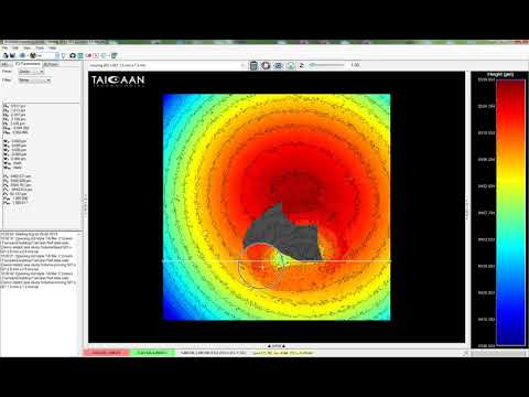
An introduction to form fitting where surface form can be fitted and removed from data to allow the examination of the residual surface. In this example a mathematically perfect sphere is removed from surface measurement of a calibration sphere (essentially a large ball bearing with a precisely measured radius). Removing a a spherical form from the measurement reveals and the error that was present in the measurement system and was undetectable before the form removal. This is a little like peeling an orange and laying the skin flat!
The first in series of longer and more in-depth case studies, this video shows how to calculate volumetric wear. The additional complication for this data is that the original surface was not flat. Because of this the correct surface form must be fitted before the correct volume of erosion can be calculated.
This case study shows how to use the data add and remove tools, then fit the correct form to the original surface, and finally isolate the region of wear to calculate the volume of the eroded material.